Bayesian Statistics: An A/B Tester’s Quick and Hype-Free Primer

How confident are you in your ability to interpret the results provided by your A/B testing tool?

Say, you’re using a tool built on Bayesian statistics, and it told you “B” has a 70% chance of beating “A” so “B” is the winner. Do you know what that means and how it should inform your CRO strategy?

In this article, you’ll learn the fundamentals of Bayesian statistics that will help you get back in control of your A/B testing, including

• An unbiased view of Bayesian statistics
• Frequentist vs Bayesian advantages and disadvantages
• The prep you need to confidently interpret and use Bayesian A/B test results while avoiding some common myth traps.

Ready? Let’s start with the basics.

What is Bayesian Statistics?

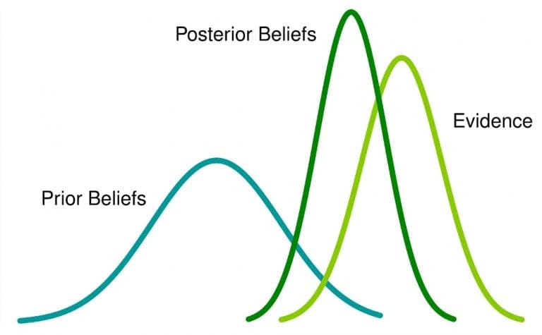
Bayesian statistics is an approach to statistical analysis that’s based on Bayes’ theorem, which updates beliefs about events as new data or evidence about those events is collected. Here, the probability is a measure of belief that an event occurs.

What this means: If you have a prior belief about an event, and get more information related to it, that belief will change (or at least be adjusted) to a posterior belief.

This is useful for understanding uncertainty or when working with lots of noisy data, such as in conversion rate optimization for ecommerce and in machine learning.

Let’s picture this:

Say, for instance, you’re watching a college grocery cart race and then an excited spectator challenges you to a bet that the dude in the red t-shirt carting the lady in a green shirt will win. You think about it and counter that the black jacket guy and black hoody girl will win instead.

Another spectator overhead and whispered a tip to you, “The red t-shirt guy won the last 3 races out of 4.” What happens to your bet? You’re not too sure anymore, right?

Supposing you also learned that the last time the black jacket guy wore his lucky sunglasses, he won. And the times he didn’t wear it, the red t-shirt guy won.

Today, you see the black jacket guy is wearing those glasses. Your belief changes again. You now have more faith in your bet, correct? In this story, you’ve updated your belief each time you got evidence of new data. That’s the Bayesian approach.

The Bayesian Origin Story

When Reverend Thomas Bayes first thought about his theory, he didn’t think it was publication-worthy. So, it remained in his notes for over a decade. It was when his family asked Richard Price to go through his notes that Price discovered the notes that formed the foundation of Bayes’ Theorem.

It started with a thought experiment for Bayes. He thought about sitting with his back to a perfectly flat and square table and having an assistant throw a ball onto the table.

The ball could land anywhere on the table, but Bayes thought he could guess where by updating his guesses with new information. When the ball landed on the table, he’d have the assistant tell him if it landed left or right, in front or behind where the previous ball had landed.

He noted that and listened as more balls landed on the table. With additional information like this, he found he could improve the accuracy of his guesses with each throw. This brought the idea of updating our understanding as we acquired more evidence from observation.

The Bayesian approach to data analysis is applied across various fields such as science and engineering, and even includes sports and law.

In online randomized controlled experiments, specifically A/B testing, you can use the Bayesian approach in 4 steps:

1. Identify your prior distribution.
2. Choose a statistical model that reflects your beliefs.
3. Run the experiment.
4. After observation, update your beliefs and calculate a posterior distribution.

You update your beliefs using a set of rules called the Bayesian algorithm.

An Example of Bayesian Statistics Applied to A/B Testing

Let’s illustrate a Bayesian A/B testing example.

Imagine we ran a simple A/B test on a Shopify store’s CTA button. For “A”, we use “Add to Cart” and for “B”, we use “Add to Your Basket”.

Here’s how a frequentist will approach the test.

There are two alternative worlds: One where A and B aren’t different, so the test won’t show any difference in conversion rate. That’s the null hypothesis. And in the other world, there’s a difference, so one button will perform better than the other.

The frequentist will assume we live in world 1 where there’s no difference in CTA buttons, that is, assuming the null hypothesis is true. And then they’ll try to prove that wrong to a pre-determined level of certainty called the significance level.

But this is how a Bayesian will approach the same test:

They start with a prior belief that both buttons A and B have equal chances to produce a conversion rate between 0 and 100%. So, there’s button equality right out of the gate — both have a 50% chance of being the top performer.

Then the test begins and data is gathered. From observing new information, Bayesian A/B testers will update their knowledge. So, if B is showing promise, they can reach a posterior belief based on that observation saying, “B has a 61% chance of beating A”.

There are core differences between the two methods.

That’s why it’s important for us to keep an unbiased approach to Bayesian A/B testing.

Most Bayesian A/B testing tools — maybe for marketing purposes — take an extreme anti-frequentist stance and push the argument that Bayesian is better at telling you which variant is more “profitable”.

But does any single statistical approach to A/B testing own the exclusive rights to insights?

If one pushes the Bayesian argument further, they may be faced with studies where the respondents say they want to know what is the best course of action or that they want to maximize profits or something similar. This puts the question firmly in decision-theoretic territory — something neither Bayesian inference nor frequentist inference can have a direct say in.

Georgi Georgiev, creator of Analytics-toolkit.com and author of “Statistical Methods in Online A/B Testing”

We’ll take a brief dive into these details in sections ahead. For now, let’s make the rest of this primer easy to grasp.

A Short Glossary of Bayesian Terms that Matter to A/B Testers

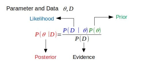
Bayesian Inference

Bayesian inference is updating the probability for a hypothesis with new data. It’s built around beliefs and probabilities.

Bayesian inference leverages conditional probability to help us understand how data impacts our beliefs. Let’s say we start with a prior belief that the sky is red. After looking at some data, we would soon realize that this prior belief is wrong. So, we perform Bayesian updating to improve our incorrect model about the color of the sky, ending up with a more accurate posterior belief.

Michael Berk in Towards Data Science

Conditional Probability

Conditional probability is the probability of an event given that another event occurred. That is, the probability of A under the condition B.

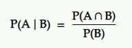
Translation: The probability of an event A happening given another event B is equal to the probability of B and A happening together divided by the probability of event B.

Probability Distribution/Likelihood Distribution

Likelihood distributions are distributions that show how likely your data will assume a specific value.

Where your data can assume multiple values, for instance, a category like colors which could be gray, red, orange, blue, etc., your distribution is multinomial. For a set of numbers, the distribution might be normal. And for data values that could either be yes/no or true/false, it would be binomial.

Prior Belief Distribution

Or prior probability distribution, simply called prior, expresses your belief before you got evidence of new data. So, it’s an expression of your initial belief which you’re going to update after considering some evidence ‌using Bayesian analysis (or inference).

Conjugacy

First of all, conjugate refers to being joined together, usually in pairs. In Bayesian probability theory, conjugacy is assuming the prior is conjugate to the likelihood.

If the posterior has the same functional form as the prior, then the prior is conjugate to the likelihood function. This shows how the likelihood function updates the prior distribution.

Conjugate Priors

This is linked to the definition above. If the posterior is in the same probability distribution family (or has the same functional form) as the prior probability distribution, then the prior and posterior are conjugate distributions. In this case, the prior is called the conjugate prior for the likelihood function.

They could be subjective (based on the experimenter’s knowledge), objective and informative (based on historical data), or non-informative.

Loss Function

A loss function is a way to quantify loss by measuring how bad our current estimate is. It helps us minimize loss for hypothesis testing, especially when expressing an inference that lies in a range of likely values, and support decision making with our test results.

Now that’s out of the way, we can move on.

If you’ve been around the block for a while, you’ve probably come across more than a few Frequentist vs Bayesian statistics memes.

Both sides seem to search for answers from opposite directions, but is that really the case? To understand this better (while remaining unbiased), let’s visit the Frequentists camp.

What is Frequentist Statistics?

This is the first inferential technique most people learn in statistics. Frequentist statistics calculate the probability that an event (hypothesis) occurs frequently under the same conditions.

A/B hypothesis testing using the frequentist approach follows these steps:

1. Declare some hypotheses. Typically, the null hypothesis is that the new variant “B” is not better than the original “A” while the alternative hypothesis declares the opposite.
2. Determine a sample size in advance using a statistical power calculation, unless you’re using sequential testing approaches. Use a sample size calculator which considers the statistical power, current conversion rate, and the minimum detectable effect.
3. Run the test and wait for each variation to be exposed to the pre-determined sample size.
4. Calculate the probability of observing a result at least as extreme as the data under the null hypothesis (p-value). Reject the null hypothesis and deploy the new variant to production if the p-value < 5%.

How does this compare to Bayesian? Let’s see…

Bayesian vs Frequentist A/B Testing

This is a notorious debate anywhere statistical inference is used. And to be frank, it is pointless. Both have their merits and instances where they’re the best method to use.

Contrary to what most promoters in both camps will have you think, they are similar in several ways and neither gets closer to the truth than the other — although their approaches differ.

When applied to A/B testing, for instance, no specific method will give you an absolute and accurate prediction in terms of the course of action that will cause business growth. Instead, A/B testing helps you remove the risk from decision-making.

No matter how you analyze your data – using Bayesian or Frequentist approaches – you can make moves with some level of certainty that you’re right.

And for that reason, both statistical models are valid. Bayesian may have a speed advantage but is more computationally demanding than Frequentist.

Check out other differences…

The Frequentist Framework

Most of us are familiar with the frequentist approach from introductory statistics courses. We defined the methodology above — from declaring the null hypothesis, determining sample size, gathering data via a randomized experiment, and finally observing a statistically significant result.

In Frequentism, we view probability as fundamentally related to the frequencies of repeated events. So, in a fair coin toss, a Frequentist believes that if they guess frequently enough, they’ll get heads right 50% of the time and the same for tails.

The Bayesian Framework

While the frequentist approach treats the population parameter for each variant as an (unknown) constant, the Bayesian approach models each parameter value as a random variable with some probability distribution.

Here, you calculate probability distributions (and thus expected values) for the parameters of interest directly.

And in order to model the probability distribution for each variant, we rely on Bayes’ rule to combine the experiment results with any prior knowledge we have about the metric of interest. We can simplify the calculations by using a conjugate prior.

Alex Birkett summarized the Bayesian algorithm this way:

• Define the prior distribution that incorporates your subjective beliefs about a parameter. The prior can be uninformative or informative.
• Gather data.
• Update your prior distribution with the data using Bayes’ theorem (though you can have Bayesian methods without explicit use of Bayes’ rule—see non-parametric Bayesian) to obtain a posterior distribution. The posterior distribution is a probability distribution that represents your updated beliefs about the parameter after having seen the data.
• Analyze the posterior distribution and summarize it (mean, median, sd, quantiles…).

In short, the Bayesian experimenter focuses on their own perspective and what probability means to them. Their opinion evolves with observed data. Frequentists, on the other hand, believe that the right answer is out there somewhere.

Understand that the Frequentist vs Bayesian debate doesn’t impact post A/B testing analysis all that much. The major differences between the two camps are more related to what can be tested.

Probability statistics are generally not used to any great extent in subsequent analysis. The Bayesian-Frequentist argument is more applicable regarding the choice of the variables to be tested in the A/B paradigm, but even there most A/B testers violate the hell out of research hypotheses, probability, and confidence intervals.

 Dr. Rob Balon to CXL

Georgi further elaborates:

There are multiple online Bayesian calculators and at least one major A/B testing software vendor applying a Bayesian statistical engine which all use so-called non-informative priors (a bit of a misnomer, but let’s not dig into this). In most cases the results from these tools coincide numerically with results from a frequentist test on the same data. Let us say the Bayesian tool will report something like ‘96% probability that B is better than A’ while the frequentist tool will produce a p-value of 0.04 which corresponds to a 96% confidence level.

In a situation like the above, which is far more common than some would like to admit, both methods will lead to the same inference and the level of uncertainty will be the same, even if the interpretation is different.

What would a Bayesian say about this result? Does it turn the p-value into a proper posterior probability when viewing a scenario in which there is no prior information? Or are all these applications of Bayesian tests misguided for using a non-informative prior per se?

There really isn’t a need to choose a camp and find a spot behind cover to throw stones at the other camp. There’s even evidence that both frameworks produce the same results. No matter the road you choose, the destination is probably going to be the same. It depends on how you can get there with Frequentist vs Bayesian.

For instance:

1. Some data shows Bayesian testing is faster and the preferred choice for interactive experiments:
   
   Since the Bayesian paradigm allows experimenters to formally quantify belief and incorporate additional knowledge, it is faster than traditional statistical analysis.
   
   In a Bayesian A/B testing simulation, when the decision criterion was adjusted (i.e., increasing the tolerance for mistakes), 75% of the experiments concluded within 22.7% of the observations required by the traditional approach (at a 5% significance level). And it recorded only a 10% type II error.
2. Bayesian is also considered more forgiving, while Frequentist is risk-averse:
   
   While many Frequentist tests use a statistical significance of 95%, Bayesians can be satisfied with less than that. If a variant has a 78% chance of beating the control, depending on the expected loss, it could be a sound decision to ‌deploy that variant.
   
   If you’re wrong and the expected loss is less than a percent, that’s pretty insignificant damage for many businesses. This scrappy approach may be better suited to quick decision-making in very low-risk scenarios.
3. However, Bayesian simulations and calculations are computation heavy:
   
   Frequentist, on the other hand, is pen- and paper-based. Caveat: If your A/B testing tool uses Bayesian and you don’t know what assumptions are being added to your data, then you can’t rely on the “answer” your vendor gives you. Take it with a pinch of salt. And run your own analysis.

It’s not all sunshine and rainbows with Bayesian. Like Georgi points out with this list of questions:

• “Do you want to get the product of the prior probability and the likelihood function?”
• “Do you want the mixture of prior probabilities and data as an output?”
• “Do you want subjective beliefs mixed with the data to produce the output?” (if using informative priors)
• “Would you be comfortable presenting statistics in which there is prior information assumed to be highly certain mixed in with the actual data?”

These are all aspects of Bayesian statistics, in layman’s terms.

What Does Bayesian Statistics Actually Tell You in A/B Testing?

You designed your A/B test to give insights into how a change affects your metric of interest, such as the conversion rate or revenue per visitor.

When you use a tool that works with Bayesian statistics, it’s important to understand what your results mean because “B is the winner” doesn’t mean exactly what most people think it does.

It’s a convenient way to present results, but that isn’t what your test revealed. Instead, the answers you want are in posterior comparisons of “A” and “B”.

Here are the 3 methods of comparison:

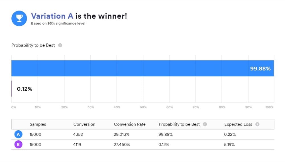
Probability to Be the Best (P2BB)

In Bayesian A/B testing, this shows each variant’s probability to be best. Whichever one has the highest probability is your most likely winner—the one that’ll probably beat out the competition.

This is calculated from a set of posterior samples of the measure of interest from the original and challenger.

So, if B has the highest probability of increasing your conversion rates, for instance, B is declared the winner.

Expected Uplift

So, if B is the winner, how much uplift should we expect from it? Would it continue to deliver the same results that we saw in the test?

That’s the insight expected uplift seeks to provide. The expected uplift of choosing B over A, given a set of posterior samples, is defined as the credible interval (or mean) of the percentage increase.

In A/B testing, we usually compare the challenger against the control. So, if the challenger lost, it’s represented in negative values (like -11.35%) and positive values (like +9.58%) if it won.

Expected Loss

Since there isn’t a 100% probability that B is better than A, then there’s a chance of recording a loss if you choose B over A. This is represented as expected loss and, just as with expected uplift, it is expressed from the point of view of the challenger against the control.

It tells you the risk of choosing your P2BB variant (i.e., the declared winner).

Before we dive into the myths, a massive thank you to analytics legend Georgi Georgiev. His in-depth analyses of frequentist vs Bayesian inference and Bayesian probability and statistics in A/B testing inspired the next section.

What Bayesian Statistics Can’t Do (Despite A/B Testing Tool Vendor Claims)

Bayesian methods often get pitched as faster, more flexible, and easier to use than Frequentist approaches.

That pitch usually includes claims like “Bayesian tests require smaller sample sizes” or “you can peek whenever you want and stop early without consequences.”

Both claims are misleading. Let’s clear up the common misconceptions about Bayesian statistics in A/B testing:

The “Faster Results” Myth

Bayesian inference continuously updates as new data arrives. That makes it feel faster, because you can always look at the current posterior. But that doesn’t mean you’re reaching valid conclusions with less data.

With large samples and uninformative priors, Bayesian and Frequentist methods converge to essentially the same result (a principle formalized in the Bernstein-von Mises theorem).

And Frequentist group-sequential tests, when designed properly, can cut expected sample size by ~15-30% (sometimes more under strong effects), shortening test times, while maintaining error control.

Speed comes from good test design, not from picking Bayesian over Frequentist.

The “Safe to Peek Anytime” Myth

A common misconception is that Bayesian methods are immune to optional stopping. The argument goes: because the posterior updates with every new data point, you can peek whenever you want.

The reality is more nuanced. Some Bayes factors and posteriors are invariant to stopping under strict assumptions. But in practice, most A/B testing relies on default or pragmatic priors and composite hypotheses. Under those conditions, the supposed robustness can break down, and the posterior can become miscalibrated, leading to biased decisions.

Leading Bayesians emphasize that the stopping rule is still part of the data-generating process. Ignoring it risks overly optimistic conclusions, just as in Frequentist testing.

Where Vendors Oversell (and Users Misinterpret)

Bayesian critics like Georgi Georgiev have documented how commercial platforms sometimes bend Bayesian outputs into marketing points:

• Hidden priors: Some vendors set priors or utility functions without disclosing them, making it impossible for users to judge or adjust assumptions.
• “Probability to be best” confusion: Some CRO tools show a “probability to beat baseline” metric. Many users expected it to shrink toward zero in an A/A test as data accumulated. Instead, it stayed around 50% — a correct Bayesian result, but far from intuitive.
• Subjective priors as levers: Bayesian analysis allows priors to encode past knowledge, but in the wrong hands, they can be chosen to generate any result you want. Without transparency, that flexibility undermines trust.
• Treating Bayesian output as objective truth: Bayesian results mix data with prior beliefs. They are decision tools, not mirrors of an underlying “objective state of nature.”

The Bottom Line Is…

Bayesian testing provides powerful, intuitive framing: probabilities you can act on. But it doesn’t remove the need for rigor.

Priors matter, stopping rules matter, and sample size still matters. Vendors that suggest otherwise risk pushing teams into decisions built on shaky ground.

So, Should You Pick Bayesian or Frequentist? There is a Place for Both.

There is no need to pick a side. Both methods have their place. For example, a long-term project that uses updated priors and needs quick results fairs better with the Bayesian approach.

The Frequentist method, on the other hand, is best suited for projects that require a significant amount of repeatability in their results. Such as in writing software that many people with many data sets will use.

As Cassie Kozyrkov, Head of Decision Intelligence at Google, says, “Statistics is the science of changing your mind under uncertainty”.

In her Bayesian vs Frequentist Statistics summary video, she said:

“You can take that Frequentist and Bayesian debate and collapse it all down to what you’re changing your mind about. Frequentists change their mind about actions, they have a preferred default action — maybe they don’t have any beliefs — but they have an action that they like under ignorance and then they ask, “Does my evidence [or data] change my mind about that action?” “Do I feel ridiculous doing it based on my evidence?”

Bayesians on the other hand, change their minds in a different way. They start with an opinion, a mathematically-expressed personal opinion, called a prior, and then they ask, “What is the sensible opinion I should have after I incorporate some evidence?” And so Frequentists change their mind about actions, Bayesians change their minds about beliefs.

And depending on how you want to frame your decision-making, you might prefer going with one camp versus the other.”

In the end, we’re all heading towards similar conclusions — the difference is in how those conclusions are presented to you.

If frequentist and Bayesian inference were programming functions, with inputs being statistical problems, then the two would be different in what they return to the user. The frequentist inference function would return a number, representing an estimate (typically a summary statistic like the sample average etc.), whereas the Bayesian function would return probabilities.

Excerpt from the book “Probabilistic Programming & Bayesian Methods for Hackers

What isn’t quite right is the claim that one gives more practical results than the other.

Key Takeaway

Bayesian statistics in A/B testing consists of 4 distinct steps:

1. Identify your prior distribution
2. Choose a statistical model that reflects your beliefs
3. Run the experiment
4. Use the results to update your beliefs and calculate a posterior distribution

Your results will point you towards insightful probabilities. So you’ll know which variant has the highest probability to be the best, your expected loss, and your expected uplift.

These are usually interpreted for you by most A/B testing tools using Bayesian statistics. But a thorough experimenter will perform a post-test analysis to understand those results better.

Because you’ve made it this far, here’s a fun fact for you: You know the portrait of Thomas Bayes everyone is familiar with? This one:

Nobody is 100% sure that’s him.