Type I and Type II Errors: The Inevitable Errors in Optimization

Type I and type II errors happen when you erroneously spot winners in your experiments or fail to spot them. With both errors, you end up going with what appears to work or not. And not with the real results.

Misinterpreting test results doesn’t just result in misguided optimization efforts but can also derail your optimization program in the long term.

The best time to catch these errors is before you even make them! So let’s see how you can avoid running into type I and type II errors in your optimization experiments.

But before that, let’s look at the null hypothesis… because it’s the erroneous rejection or non-rejection of the null hypothesis that causes type I and type II errors.

The Null Hypothesis: ​H0

When you hypothesize an experiment, you don’t directly jump to suggest that the proposed change will move a certain metric.

You start by saying that the proposed change won’t impact the concerned metric at all — that they’re unrelated.

This is your null hypothesis (H0). H0 is always that there is no change. This is what you believe, by default… until (and if) your experiment disproves it.

And your alternative hypothesis (Ha or H1) is that there is a positive change. H0 and Ha are always mathematical opposites. Ha is the one where you expect the proposed change to make a difference, it is your alternative hypothesis — and this is what you’re testing with your experiment.

So, for instance, if you wanted to run an experiment on your pricing page and add another payment method to it, you’d first form a null hypothesis saying: The additional payment method will have no impact on sales. Your alternate hypothesis would read: The additional payment method WILL increase sales.

Running an experiment is, in fact, challenging the null hypothesis or the status quo.

Type I and type II errors happen when you erroneously reject or fail to reject the null hypothesis.

Understanding Type I Errors

Type I errors are known as false positives or Alpha errors.

In a type I error instance of hypothesis testing, your optimization test or experiment *APPEARS TO BE SUCCESSFUL* and you (erroneously) conclude that the variation you’re testing is doing differently (better or worse) than the original.

In type I errors, you see lifts or dips — that are only temporary and won’t likely maintain in the long term — and end up rejecting your null hypothesis (and accepting your alternative hypothesis).

Erroneously rejecting the null hypothesis can happen for various reasons, but the leading one is that of the practice of peeking (i.e., looking at your results in the interim or when the experiment’s still running). And calling the tests sooner than the set stopping criteria is reached.

Many testing methodologies discourage the practice of peeking as looking at interim results could lead to wrong conclusions resulting in type I errors.

Here’s how you could make a type I error:

Suppose you’re optimizing your B2B website’s landing page and hypothesize that adding badges or awards to it will reduce your prospects’ anxiety, thereby increasing your form fill rate (resulting in more leads).

So your null hypothesis for this experiment becomes: Adding badges has no impact on form fills.

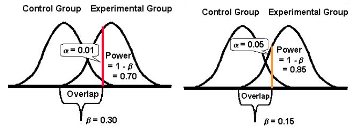
The stopping criteria for such an experiment is usually a certain period and/or after X conversions happen at the set statistical significance level. Conventionally, optimizers try to hit the 95% statistical confidence mark because it leaves you with a 5% chance of making the type I error that’s considered low enough for most optimization experiments. In general, the higher this metric is, the lower are the chances of making type I errors.

The level of confidence that you aim for determines what your probability of getting a type I error (α) will be.

So if you aim for a 95% confidence level, your value for α becomes 5%. Here, you accept that there’s a 5% chance that your conclusion could be wrong.

In contrast, if you go with a 99% confidence level with your experiment, your probability of getting a type I error drops to 1%.

Let’s say, for this experiment, that you get too impatient and instead of waiting for your experiment to end, you look at your testing tool’s dashboard (peek!) just a day into it. And you notice an “apparent” lift — that your form fill rate has gone up by a whopping 29.2% with a 95% level of confidence.

And BAM…

… you stop your experiment.

… reject the null hypothesis (that badges had no impact on sales).

… accept the alternative hypothesis (that badges boosted sales).

… and run with the version with the awards badges.

But as you measure your leads over the month, you find the number to be nearly comparable to what you reported with the original version. The badges didn’t matter so much after all. And that the null hypothesis was probably rejected in vain.

What happened here was that you ended your experiment too soon and rejected the null hypothesis and ended up with a false winner — making a type I error.

Avoiding Type I Errors in Your Experiments

One sure way of lowering your chances of hitting a type I error is going with a higher confidence level. A 5% statistical significance level (translating to a 95% statistical confidence level) is acceptable. It’s a bet most optimizers would safely make because, here, you’ll fail in the unlikely 5% range.

In addition to setting a high confidence level, running your tests for long enough is important. Test duration calculators can tell you for how long you must run your test (after factoring in things like a specified effect size among others). If you let an experiment run its intended course, you significantly reduce your chances of encountering the type 1 error (given you’re using a high confidence level). Waiting until you reach statistically significant results ensures that there is only a low chance (usually 5%) that you rejected the null hypothesis erroneously and committed a type I error. In other words, use a good sample size because that’s crucial to getting statistically significant results.

Now that was all about type I errors that are related to the level of confidence (or significance) in your experiments. But there is another type of error too that can creep into your tests — the type II errors.

Understanding Type II Errors

Type II errors are known as false negatives or Beta errors.

In contrast to the type I error, in the instance of a type II error, the experiment *APPEARS TO BE UNSUCCESSFUL (OR INCONCLUSIVE)* and you (erroneously) conclude that the variation you’re testing isn’t doing any different from the original.

In type II errors, you fail to see the real lifts or dips and end up failing to reject the null hypothesis and rejecting the alternative hypothesis.

Here’s how you could make the type II error:

Going back to the same B2B website from above…

So suppose this time you hypothesize that adding a GDPR compliance disclaimer prominently at the top of your form will encourage more prospects to fill it out (resulting in more leads).

Therefore, your null hypothesis for this experiment becomes: The GDPR compliance disclaimer doesn’t impact form fills.

And the alternative hypothesis for the same reads: The GDPR compliance disclaimer results in more form fills.

A test’s statistical power determines how well it can detect differences in the performance of your original and challenger versions, should any deviations exist. Traditionally, optimizers try to hit the 80% statistical power mark because the higher this metric is, the lower are the chances of making type II errors.

Statistical power takes a value between 0 and 1 (and is often expressed in %) and controls the probability of your type II error (β); it’s calculated as: 1 – β

The higher the statistical power of your test, the lower will be the probability of encountering type II errors.

So if an experiment has a statistical power of 10%, then it can be quite susceptible to a type II error. Whereas, if an experiment has a statistical power of 80%, it will be far less likely to make a type II error.

Again, you run your test, but this time you don’t notice any significant uplift in your form fills. Both versions report near similar conversions. Because of which, you stop your experiment and continue with the original version without the GDPR compliance disclaimer.

However, as you dig deeper into your leads data from the experiment period, you find that while the number of leads from both versions (the original and the challenger) seemed identical, the GDPR version did get you a good, significant uptick in the number of leads from Europe. (Of course, you could have used audience targeting to show the experiment only to the leads from Europe – but that’s another story.)

What happened here was that you ended your test too early, without checking if you had attained sufficient power  — making a type II error.

Avoiding Type II Errors in Your Experiments

To avoid type II errors, run tests with high statistical power. Try to configure your experiments so you can hit at least the 80% statistical power mark. This is an acceptable level of statistical power for most optimization experiments. With it, you can ensure that in 80% of the cases, at least, you’ll correctly reject a false null hypothesis.

To do this, you need to look at the factors that add to it.

The biggest of these is the sample size (given an observed effect size). The sample size ties directly to the power of a test. A huge sample size means a high power test. Underpowered tests are very vulnerable to type II errors as your chances of detecting differences in the results of your challenger and original versions reduce greatly, especially for low MEIs (more on this below). So to avoid type II errors, wait for the test to accumulate sufficient power to minimize type II errors. Ideally, for most cases, you’d want to reach a power of at least 80%.

Another factor is the Minimum Effect of Interest (MEI) that you target for your experiment. MEI (also called MDE) is the minimum magnitude of the difference that you would want to detect in your KPI in question. If you set a low MEI (eyeing a 1.5% uplift, for example), your chances of encountering the type II error increase because detecting small differences needs substantially bigger sample sizes (to attain sufficient power).

And finally, it’s important to note that there tends to be an inverse relationship between the probability of making a type I error (α) and the probability of making a type II error (β). For example, if you decrease the value of α to lower the probability of making a type I error (say you set α at 1%, meaning a confidence level of 99%), the statistical power of your experiment (or its ability, β, of detecting a difference when it exists) ends up reducing too, thereby increasing your probability of getting a type II error.

Being More Accepting of Either of the Errors: Type I and II (& Striking a Balance)

Lowering the probability of one type of error increases that of the other type (given all else remains the same).

And so you need to take the call on what error type you could be more tolerant toward.

Making a type I error, on one hand, and rolling out a change for all your users could cost you conversions and revenue — worse, could be a conversion killer too.

Making a type II error, on the other hand, and failing to roll out a winning version for all your users could, again, cost you the conversions you could have otherwise won.

Invariably, both the errors come at a cost.

However, depending on your experiment, one might be more acceptable to you over the other.  In general, testers find the type I error about four times more serious than the type II error.

If you’d like to take a more balanced approach, statistician Jacob Cohen suggests you should go for a statistical power of 80% that comes with “a reasonable balance between alpha and beta risk.” (80% power is also the standard for most testing tools.)

And as far as the statistical significance is concerned, the standard is set at 95%.

Basically, it’s all about compromise and the risk level that you’re willing to tolerate. If you wanted to truly minimize the chances of both the errors, you could go for a confidence level of 99% and a power of 99%. But that would mean you’d be working with impossibly huge sample sizes for periods seeming eternally long. Besides, even then you’d be leaving some scope for errors.

Every once in a while, you WILL conclude an experiment wrongly. But that’s part of the testing process — it takes a while to master A/B testing statistics. Investigating and retesting or following up on your successful or failed experiments is one way to reaffirm your findings or discover that you made a mistake.